L3 Daily Algorithm

Understanding the L3 Gridding

Before one can understand the L3 algorithm and how the L2 input data is gridded in L3; it's best to review the stored geolocation of the L2 (input) products - since that input L2 geolocation is used to place the input data on the L3 grid.

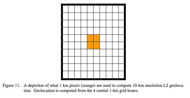
Computation of geolocation in L2 atmosphere products MODIS Atmosphere Level 2 (L2) HDF files always have geolocation arrays stored at either 5-km or alternatively 10-km resolution. The Aerosol (04_L2) product contains 10-km resolution geolocation and 10-km retrieval data. All other Atmosphere products used as input into L3 (Water Vapor (05_L2), Cloud (06_L2), Profiles (07_L2)) contain 5-km resolution geolocationand either 1-km or alternatively 5-km retrieval data. Retrieval data for 10-km resolution L2 products like aerosol properties are generated from 10×10 1-km L1B input pixels. The geolocation for these 10×10 km resolution products is computed by averaging the geolocation for the four central
(column, row) pairs: (5,5), (5,6), (6,5), (6,6), as shown in the Figure below.

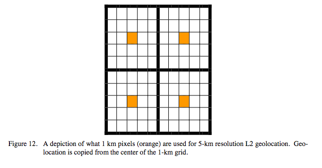
Retrieval data for 5-km resolution L2 data products is generated from 5×5 1-km L1B input pixels. Retrieval data for 1-km resolution L2 data products is computed at the native 1 km L1B input pixel resolution. For L2 HDF files containing both of these cases, the geolocation is stored at 5-km resolution. The 5×5 km geolocation is copied from center (column,row) pair: (3,3), as shown in the Figure below.  Note that the 2×2 5-km grid area (the outer boundary the Figure above) matches the 10km grid area (the outer boundary in Figure at the top of this page, exactly.

A Note about Dropped pixels in L2 products

One additional characteristic should be noted here. A MODIS scan is 1354 1-km pixels in width. For 5 and 10 km resolution L2 products, the last 4 pixels in each MODIS scan are effectively dropped when performing retrievals (a pre-launch decision made by the L2 development teams). For example, for 5 km cloud top property parameters, no retrieval is made for the last 4 (hanging) pixels in each scan line. This also impacts the geolocation (latitude
and longitude) arrays where there is not geolocation computed or stored for the last 4 pixels.  To make this clearer, even though there are 1354 1-km pixels in a scanline, there are only 270 5-km cross-scan geolocation grid points and data retrievals in 5-km L2 products (and 135 geolocation grid points and data retrievals in 10-km L2 products). Therefore, in all 5-km and 10-km L2 products (and L3 products derived from those L2 products), a very tiny
amount of potential data at the far edge of each MODIS swath is not used, however due to the 1° × 1° averaging in L3, this is more of an issue in 5-km and 10-km L2 products than in 1° × 1° L3.
 

Sampling the L2 Pixels in L3

Sampling of L2 input data for computation of L3 statistics is always performed whenever the input L2 pixel resolution is at a different (finer) resolution than the stored geolocation within the L2 input product file. This occurs in all parameters noted by the red boxes in the Table 1. So for cases where L2 data are at 1-km resolution and geolocation is stored at 5-km, the L3 software samples the 1-km L2 data every 3rd column and every 3rd row. This ensures the L2 data pixel matches exactly the stored geolocation. (Refer back to Figure 11 and note the orange-colored 1 km pixel.) Note that starting in collection 5, this sampling convention was changed (see section 2.2.1 for details). Table 1. L2 parameters that are impacted by sampling (note that counts are approximated for nadir view at the Equator). There were three reasons why sampling was done in the L3 production: (i) it removed the need to compute geolocation for all (input) 1-km L2 pixels, greatly simplifying the L3 operational software, (ii) fewer L2 pixels needed to be read and operated on, reducing the operational run and CPU time, and (iii) it was found that sampling causes minimal impact of computed statistics at the operational L3 grid resolution of 1° × 1°. 2.2.1. Sampling modification to avoid dead detectors A software modification was introduced in Collection 5 (the latest MODIS Atmosphere data version available as of calendar year 2008), which offset slightly the L2 data point sampled. This patch only impacts L3 data that are derived from sampled L2 data and includes Water Vapor (05_L2), Cirrus Detection and Cloud Optical Property (06_L2) parameters (see Table 1), all of which are computed and stored at 1 km resolution in the L2 files but are sampled at 5 km resolution for computation of L3 gridded statistics. In these cases, the geolocation matches the 1-km area corresponding to the orange square in Figure 13. This corresponds to the 1-km pixel located in column 3, row 3. However, the actual L2 data are sampled from the blue square (1 km pixel located in column 3, row 4). In other words, L2 data from MODIS detectors 4 and 9 are sampled (instead of detectors 3 and 8) in the 10-detector set. This patch was necessary because in some critical MODIS spectral bands on the Aqua platform, detectors 3 and 8 both died (that is, always contained missing data); so a shift to adjacent detectors was necessary to prevent many subsampled products from being completely missing (fill values) in L3. Figure 13. A shift in the L2 “sampling pixel” for 5 km L2 input products was implemented to prevent dead detectors from causing missing L3 data in Collection 5 (Orange = Collection 4 sampling at the center of the 5 × 5 (column 3, row 3), Blue = Collection 5 Sampling at (column 3, row 4) slightly off center of the 5 × 5 grid box. In other words, in Collection 4, L2 pixels from detectors 3 & 8 were sampled; in Collection 5, L2 pixels from detectors 4 & 9 were sampled. The choice of which alternate pair of detectors to pick [(1 & 6), (2 & 7), (4 & 9), or (5 & 10)] was made to both minimize errors in geolocation as well as inherent detector errors. It turned out that detectors 4 and 9 had the dual benefit of: (i) being immediately adjacent to the geolocation pixel so only a 1 km geolocation error was introduced, and (ii) both detectors 4 and 9 were well behaved and had small residual errors when compared to averages taken over the entire 5 × 5 km area (Oreopoulos 2005). Even though the change in start detector (from the 3rd to the 4th) was prompted by the failure of Aqua MODIS detectors 3 and 8 in band 6 (1.64 µm), the change was extended to Terra data as well after a study showed that Terra detector pairs 4 and 9 provided the most representative results over a 5 km grid cell (Oreopoulos 2005) and it was thought that matching the logic between Terra and Aqua versions of the L3 software was prudent. Computation of L3 Daily Statistics The quality of a Level 2 product can be (i) inherited from the L1B radiances, or (ii) associated with the retrieval process. The pixel-based L1B validity flags comprising information on dead and saturated detectors, calibration failure, etc., are examined by L2 algorithms for determination of the radiometric status of each pixel. This information can prevent further calculations from being performed if the “valid L1B input data” criteria are not met by the given algorithm. The granule-level (L1B) QA metadata provide summary information for valid and saturated Earth view observations, and can be useful in screening a granule of data. Details about MODIS L1B QA flags can be found on the MCST web site (www.mcst.ssai.biz/L1B/L1B_docs). The structure and information content of MODIS Atmosphere L2 runtime QA are detailed in the QA Plan available on the MODIS Atmosphere web site (atmosphere-imager.gsfc.nasa.gov/reference_atbd.php). It should be noted that runtime QA flags are only found in Level 2 (L2) Atmosphere products. Level 3 (L3) Atmosphere products contain no runtime QA flags; however L2 runtime QA flags are used in L3 to compute (aggregate and QA weight) statistics in L3. Aggregation and QA weighting of statistics All L3 products (Daily, Eight-Day, and Monthly) make use of Aggregation and QA weighting capabilities. Aggregation and QA weighting information is read in from and based upon L2 (input) QA bit flag SDSs. It should also be noted that L3 statistics can be both aggregated and QA weighted; how- ever only a single aggregation and/or QA weighting can be performed for any given output L3 SDS (a limitation in the L3 operational software). Aggregation of statistics based on physical properties For some parameters, it is useful to aggregate results into L3 SDSs based on a physical characteristic of the parameter or of the scene. Aggregation refers to the ability to separate L2 input pixel information into various scientifically relevant categories such as liquid water clouds only, ice clouds only, daytime only, nighttime only, clear sky only, dusty scene only, smoky scene only, etc. This aggregation utilizes L2 “Runtime QA Flags” that are designed to convey information on retrieval processing path, input data source, scene characteristics, and the estimated quality of the physical parameters retrieved. In addition, this broad group of flags also includes Cloud Mask flags (initially derived at 1 × 1 km resolution) that may be recomputed at the spatial resolution of the L2 retrieval for the determination such scene characteristics as cloudy/clear, land surface type, sunglint, day/night, and snow/ice. In L3 these statistics are noted by a suffix to the SDS name (_Liquid, _Dust, etc.). Additional detail and documentation are always provided in the local attribute “long_name” attached to each L3 SDS within the HDF file. Table 2 lists the various L2 products that have this aggregation information available for use in L3. QA weighting of statistics based on confidence QA weighting refers to the ability to weight more heavily what are expected to be more reliable L2 input pixels in the computation of L3 statistics. There are four levels of “reliability” or “confidence” set by the L2 QA Confidence Flags. These four levels are: No Confidence or Fill (QA = 0), Marginal Confidence (QA = 1), Good Confidence (QA = 2), or Very Good Confidence (QA = 3). QA weighted statistics always have the identifying string “QA” somewhere in the Scientific Data Set (SDS) name (for example: “QA_Mean”). Additional detail on the flags used to perform the QA weighting can be found in the local attributes that begin with the string “QA.” Only six of the derived L3 Daily statistics have the ability to be QA weighted: Mean, StandardDeviation, LogMean, LogStandardDeviation, MeanUncertainty, and LogMeanUncertainty. A seventh related statistic, the Confidence Histogram, does not actually “weight” the statistics by confidence, but does compute (sum) the counts of the various confidence categories so the relative populations of QA confidence categories can be analyzed. QA Weighted Statistics are computed by weighting all L2 pixels by their QA confidence flag value given in Table 3, using the equation below: L3 QA Weighted Statistic = ∑ di wi / ∑ wi, (1) where, L2 data value = di, L2 QA value = wi (weight = 0, 1, 2, 3) Table 3. The weighting given in L3 QA-weighted statistical computations to various L2 QA Confidence categories. So while all non-fill QA = 0 pixels are included in regular statistics; they are screened (removed) from QA weighted statistics. For example: if a L3 1° grid cell had three L2 pixels to average, and one L2 pixel had a QA Confidence value of 3, one had a value of 1, and one had a value of 0; then L2 pixel with QA = 3 will have three times more weighting when computing the L3 gridded mean than the QA = 1 pixel, and the QA = 0 pixel would not be used at all in the QA weighted mean (it would however still be used in the regular mean, where no QA weights are applied). This technique allows for the creation of L3 (QAweighted) statistics that can selectively exclude no confidence (or experimental) L2 results. Confidence Histograms are computed by totaling the pixel counts (note these may be subsampled, see Table 1) in each L3 1° grid cell of a L2 parameter that fell in one of the four confidence categories described above. Finally note that for regular (non QA-weighted) statistics, all L2 pixels are given equal weight in the L3 statistical computation; and QA = 0 (no confidence) non-fill L2 input pixels are included in the computation of statistics. Types of daily statistics computed A total of 14 different general types of statistics are computed in the daily product. These general statistical categories are Simple Statistics, QA-weighted Statistics, Fraction Statistics, Log Statistics, Uncertainty Statistics, Regression Statistics, Pixel Counts, Confidence Histograms, Marginal Histograms, and Joint Histograms. Statistics in the Daily file are always based on the set of L2 input pixels read from the four L2 input product files: Aerosol, Water Vapor, Cloud, and Atmospheric Profile. Users should note that, in addition to regular simple statistics, L2 QA Confidence flags are also ignored in the L3 computation of pixel count, histogram, joint histogram, and regression statistics. Simple statistics • Mean. Statistics always have the Scientific Data Set (SDS) name suffix “_Mean” and are computed by taking an unweighted average of L2 pixels (sometimes sampled, see Table 1) within a given 1° L3 grid cell. • Standard Deviation. Statistics always have the Scientific Data Set (SDS) name suffix “_Standard_Deviation” and are computed by calculating an unweighted standard deviation of all L2 pixels (sometimes sampled, see Table 1) within a given 1° L3 grid cell. • Minimum. Statistics always have the Scientific Data Set (SDS) name suffix “_Minimum” and are computed by finding the minimum value of L2 pixels (sometimes sampled, see Table 1) within a given 1° L3 grid cell. • Maximum. Statistics always have the Scientific Data Set (SDS) name suffix “_Maximum” and are computed by finding the maximum value of L2 pixels (sometimes sampled, see Table 1) within a given 1° L3 grid cell. QA-weighted simple statistics • QA_Mean. Level 2 Confidence QA Flags that indicate the quality of each L2 pixel are used to weight the pixels when computing the L3 mean (see Section 3.1.2 for details on QA-weighting). • QA_Standard_Deviation. Level 2 Confidence QA Flags that indicate the quality of each L2 pixel are used to weight the pixels when computing the L3 standard deviation (see Section 3.1.2 for details on QA-weighting). Fraction statistics. These statistics are only used for computing cloud fraction. • Fraction. Estimates of cloud fraction based on L2 pixel data. Some fractions are computed from QA Flags that describe the cloudiness of the scene and some directly from the L2 Cloud Fraction SDS data. Pixel count statistics. These statistics are only computed for some parameters. It is similar to a histogram computation except that instead of multiple bins there is only a single bin that covers the full range of all non-fill L2 data that are read in for each L3 1° × 1° grid cell. • Pixel Count. The count of all non-fill L2 pixel data that are read in and used to compute statistics at L3. Logarithm statistics. These statistics are only computed for cloud optical thickness (c) parameters. Because of the curvature of cloud reflectance as a function of optical thickness, the mean optical thickness of an ensemble of pixels does not correspond to the mean reflectance (or albedo) of those pixels. However, the mean of log(c) approximates the radiatively-averaged optical thickness because reflectance plotted as a function of log(c) is linear over a wide range of optical thickness (excluding small and large values). That is, the mean of log(c) gives an optical thickness that approximately corresponds to the average reflectance of the pixels that comprise the mean. The accuracy of this approximation depends on the nature of the optical thickness probability density function (PDF). Studies on the validity of this approximate for MODIS scenes have been reported by Oreopoulos et al. (2007). A similar study on ice clouds by the same authors is ongoing. • Log_Mean. L2 cloud optical thicknesses (c) are converted to base 10 logs. Thus a c of 100 would be converted to a value of 2.0, a c of 10 would be converted to a value of 1.0, a c or 1.0 would be converted to a value of 0, a c of 0.1 would be converted to a value of –1.0, and finally a c of 0.01 would be converted to a value of –2.0. So the valid range of this statistic is –2.0 to 2.0 (corresponding to data values ranging from 0.01 to 100). Once the log values of the L2 input pixel data are calculated, a daily mean value of all the log values is computed. • Log_Standard_Deviation. L2 cloud optical thicknesses (c) are converted to base 10 logs and a standard deviation value of all the L2 log values is computed. • QA_Log_Mean. L2 cloud optical thicknesses (c) are converted to base 10 logs and a QA-weighted mean value of all the L2 log values is computed (see Section 3.1.2 for details on QA-weighting). • QA_Log_Standard_Deviation. L2 cloud optical thicknesses (c) are converted to base 10 logs and a QA-weighted standard deviation value of all the L2 log values is computed (see Section 3.1.2 for details on QA-weighting). Uncertainty statistics. These statistics are only reported for a few selected Cloud Optical Property parameters. The uncertainty estimate accounts for three error sources only (instrument calibration/modeling error, surface albedo, atmospheric corrections), and as such should be considered an expected minimum uncertainty, i.e., the inclusion of additional (uncorrelated) error sources will increase the uncertainty. Daily uncertainty calculations assume all pixel-level error sources are correlated within a grid box. It should be noted that L2 uncertainties are reported in percentage (valid range 0 to 200%) – these are called relative uncertainties. In L3, uncertainties are reported as absolute uncertainties in the same units as the parameter whose uncertainty is being measured. To convert these back into relative uncertainties (%) one must divide the L3 uncertainty by the L3 mean value of the parameter in question. The conversion of relative to absolute uncertainties in the Daily (D3) file was done to make the computation of the multiday (E3 and M3) uncertainties easier to add to the multiday production software. • Mean_Uncertainty. An estimate of the absolute uncertainty that is derived from L2 pixel-level relative uncertainties. • QA_Mean_Uncertainty. An estimate of the QA-weighted absolute uncertainty that is derived from L2 pixel-level relative uncertainties (see Section 3.1.2 for details on QA-weighting). Logarithm of uncertainty statistics. An estimate of the log uncertainty that is derived from pixel-level uncertainties. • Log_Mean_Uncertainty. An estimate of the log uncertainty that is derived from pixel-level uncertainties. • QA_Log_Mean_Uncertainty. An estimate of the QA-weighted log uncertainty that is derived from pixel-level uncertainties (see Section 3.1.2 for details on QAweighting). Histogram. A distribution of L2 pixels. • Histogram. A histogram that contains pixel counts showing the distribution of nonfill L2 pixels that went into the computation of L3 statistics for each L3 grid cell. Histogram bin boundaries are set by a local attribute attached to the histogram SDS. Note that these L2 count values are sampled totals for Water Vapor, Cirrus Detection, and Cloud Optical Property parameters (See Table 1). It should also be noted that the lowest (1st) histogram bin includes L2 data points that fall on either the lowest (1st) bin boundary or the 2nd bin boundary (exactly). All subsequent bins only contain points that fall on the higher bin boundary. Any L2 data point that falls outside the specified range of bin boundaries is not counted. Histogram of confidence. A distribution of L2 pixel-level retrieval confidence. • Confidence_Histogram. A histogram that contains pixel counts showing the number of Questionable (QA = 1), Good (QA = 2), Very Good (QA = 3), and Total Level-2 Input Pixels (# non-fill L2 Pixels) that went into the computation of L3 statistics for each L3 grid cell. Note that these values are sampled totals for Water Vapor, Cirrus Detection, and Cloud Optical Property parameters (See Table 1). Joint histogram. A distribution of L2 pixels comparing one parameter against another. • Joint_Histogram. A 2-dimensional histogram that contains pixel counts showing the distribution of non-fill L2 pixels when comparing one parameter against another. Joint Histogram bin boundaries are set by a local attribute attached to the Joint_Histogram SDS in question. Note that these pixel count values are sampled totals for Cloud Optical Property parameters (See Table 1). It should be noted that only a few Cloud parameters have Joint Histograms defined. The binning logic convention is as follows: the lowest (1st) histogram bin (for both parameters) includes L2 data pixels that fall on either the lowest (1st) bin boundary or the 2nd bin boundary (exactly). All subsequent bins only contain pixels that fall on the higher bin boundary. Any L2 pixels that fall outside the specified bin boundary range are not counted. Pixels for both parameters must be defined (non-fill) and within the specified range of bin boundaries for either pixel to be binned. Joint regression. A regression fit of L2 pixels comparing one parameter against another. Note that these are only computed for a few Aerosol parameters. • Regression_Slope. A computation of the regression slope that describes the linear fit distribution of non-fill L2 pixels when comparing one parameter against another. • Regression_Intercept. A computation of the regression intercept that describes the linear fit distribution of non-fill L2 pixels when comparing one parameter against another. • Regression_R_squared. A computation of the regression r2 that describes the linear fit distribution of non-fill L2 pixels when comparing one parameter against another. • Regression_Mean_Square_Error. A computation of the regression mean squared error (MSE) that describes the linear fit distribution of non-fill L2 pixels when comparing one parameter against another.